Dimensionality Reduction
January 4, 2019 | Words by Bhaarat Sharma
CIO Level Summary
-
Modern datasets often have a large number of features which add richness, but also complexity.
-
In situations where the complexity of the data is too much either for humans to understand, or computers to process in a time efficient manner, we often want to reduce the number of features (dimensions) in the dataset.
-
When doing Dimensionality Reduction, we want to keep as much useful information as possible. The techniques described below (PCA, LDA, LASSO, RIDGE, Elastic Net, and Autoencoders) aim to mitigate issues of dimensionality while maintaining as much richness in the data as possible.
What is Dimensionality and Why do we want to reduce it?
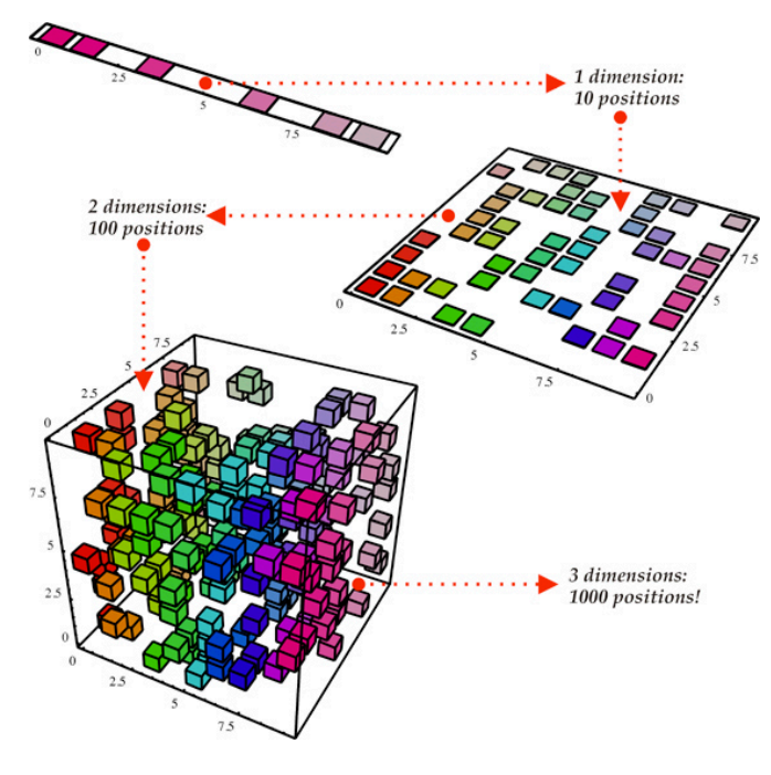
Interesting and useful datasets are often (though not always) rather large. They generally have both many observations (for example, data on 90 million homes recently listed on Zillow.com), and many features (information about each observation such as longitude, latitude, state, city, rent price, neighborhood...etc). The features of a dataset are often referred to as dimensions. A good rule of thumb for understanding that term is picturing a scatterplot of your features. If you only have two features you could plot it on a two-dimensional graph. If you had three, a three-dimensional graph...and so on.
Human brains can process 3, perhaps 4 dimensions at a time. But once you try to look at 5 let alone 100 dimensions, you’re going to struggle to observe the types of patterns that jump out at you in 2 or 3 dimensions. Dimensionality reduction is often used in order to make data more consumable to human beings. We can take 100 features and squish it down into 2 or 3 easily visualized features.
But humans are not the only issue. Even if we’re okay with the fact that we cannot easily visualize 1,000 dimensional data, we may not be able to stomach the time cost of creating a model to understand our data that will take hours--if not days or weeks--to complete. Taking data from 1,000 to 100 features doesn’t help human beings comprehend patterns and trends in the data, but it allows computers to do so much faster.
There are many different methods of dimensionality reduction, and different situations call for different methods. The first methods that we will talk about are methods of combining existing features to create a new smaller set of features.
Principal Components Analysis (PCA) and Linear Discriminant Analysis (LDA)
PCA. Principal Components Analysis takes all of your existing features (we’ll call the number of features you have, n) and creates a new set of n features. It might seem redundant to take n features and make n different ones, but these new features--called principal components--have a particularly useful characteristic. These new principal components (PCs) are created so that the first PC explains as much variance in the data as possible. Let’s take a step back and look at what this means visually.
Let’s look at this scatterplot which shows subjects’ height and weight (both z-scored).

There’s some variation in both the x and y axes. But by looking at the data, we can see that there is the most variation is in this direction. If we ignored the x and y axes and drew this line as a new axis, it would have the highest amount of variance that one axis could have.

We can then draw a new second axis perpendicular to this new one

These new axes--our principal components--are linear combinations of our old x and y values. But these principle components maximize the amount of variance explained so that the first principal component explains the most variance in the data, and the second (or nth, if you have more than 2 original features) component explains the least. The principal components are orthogonal to each other. This means they’re at 90 degree angles to each other. Practically, this means each of our PCs is uncorrelated with all the other PCs.
To find these principal components, we use eigenvalue decomposition to break the covariance matrix of all the features into its corresponding eigenvectors and eigenvalues. The eigenvectors are our new axes, or principal components. The eigenvalues give us an idea of how much of the overall variance is accounted for by each component. In general, the large the eigenvalue, the more variance the corresponding eigenvector (the PC) accounts for.
But we are trying to reduce dimensions, and PCA naturally makes n new components out of n original features. So, we want to get rid of some of the PCs while still explaining as much of the variation in the data as possible. In this case, variation means information. We could easily reduce even a 100 feature dataset to a 1 dimensional one by taking all the feature values and averaging them together to form one new score. However, this gets rid of a lot of the useful information in the data.
We can take advantage of the fact that our new PCs are ranked in order of how much variance they explain. We can choose m components (where m < n) that explain most of the variance in the data. For example, this diabetes dataset has 8 features that we can use for clustering: # of Pregnancies, Glucose Level, Blood Pressure, Skin Thickness, Insulin, BMI, Diabetes Pedigree Function, and Age.
Table 1. Example of Diabetes Data.
| Pregnancies | Glucose | BP | Skin Thick | Insulin | BMI | DPF | Age |
|---|---|---|---|---|---|---|---|
| 6 | 148 | 72 | 35 | 0 | 33.6 | 0.627 | 50 |
| 1 | 85 | 66 | 29 | 0 | 26.6 | 0.351 | 31 |
| 8 | 183 | 64 | 0 | 0 | 23.3 | 0.672 | 32 |
| 1 | 89 | 66 | 23 | 94 | 28.1 | 0.167 | 21 |
Let’s import our packages and load in our data to python (note: each feature in the csv is now z-scored).
import numpy as np
import pandas as pd
from sklearn.preprocessing import StandardScaler
from sklearn.decomposition import PCA
from sklearn.discriminant_analysis import LinearDiscriminantAnalysis
from sklearn.linear_model import Lasso, Ridge, ElasticNet
import matplotlib.pyplot as plt
from ggplot import *
from keras.layers import Input, Dense
from keras.models import Model


dia = pd.read_csv("diabetesScaled.csv")
We can run principal components analysis on this data set, and then generate a scree plot which will show us how much variance is accounted for by each principal component.
pca = PCA()
pcs = pca.fit(dia)
plt.plot(pcs.explained_variance_ratio_)
plt.xlabel('number of components')
plt.ylabel('cumulative explained variance')
plt.show()

We can see in this plot that the first Principal component accounts for almost 25% of the variance in the original data. And all together, the first 5 account for almost 90% of the original variation. We could drop almost ⅓ our our features and only lose about 10% of the original variation.
There’s no hard or fast rule for choosing the number of PCs to retain. The “elbow” methods looks at the scree plot and decides where the inflection point (or “elbow”) of the graph is, and includes all PCs before that point. Others will include any PC with an eigenvalue greater than 1, and still others will choose a proportion of variance (usually 95%+) they want to retain and keep only enough PCs to reach that proportion.
LDA. While PCA performs dimensionality reduction by finding the eigenvalues and eigenvectors of the total covariance matrix, Linear Discriminant Analysis (LDA) does something similar, but to a different kind of covariance matrix.
LDA is still interested in finding new axes that account for the most variance possible. But this time, we want to focus on between and within class variance. In our diabetes data set, we have two groups: people with a diabetes diagnosis and those without. And we’d like to know the differences between these groups, especially if it can help us classify new people as either diabetic or not.
So, LDA decomposes the combination of the within (\(S_W\); how much variation is within each group) and between (\(S_B\); how much variation there is between diabetics and non diabetics) covariance matrices.
\[S_W = \sum\limits_{i=1}^{c} S_i%0\] \[\text{where } S_i = \sum\limits_{\pmb x \in D_i}^n (\pmb x - \pmb m_i)\;(\pmb x - \pmb m_i)^T%0\] \[S_B =\sum\limits_{i=1}^{c} N_{i} (\pmb m_i - \pmb \mu) (\pmb m_i - \pmb \mu)^T%0\]The covariance matrix we decompose is \(S_w^{-1}S_B%0\) which allows us to simultaneously maximize between group variance (i.e. the groups will be far apart from each other on these new component axes), and minimize the within group variance (i.e. data points in each group will be close to other points in the group on these new component axes).
Once we’ve decomposed this matrix to get our new axes, we can keep as many, or as few components as we want, all while retaining as much information about what makes our two groups--diabetic and non-diabetic--separate from each other. This gives as a good, and less computationally expensive way of figuring out whether new patients are likely to have diabetes.
lda = LinearDiscriminantAnalysis()
lds = lda.fit(diapc, dia["Outcome"])
scores = lda.transform(diapc)
ggdf = pd.DataFrame({"score": scores.flatten(), "diabetic": list(dia["Outcome"]), "n": [1] * len(scores)})
p = ggplot(aes( x = "score", y = "n", color = "diabetic"),data = ggdf)  + geom_point() +ylim(0,2)
print(p)
When we plot the data using one component from LDA, we can see that the groups are pretty well separated using this new axis.

LASSO and RIDGE Regression, and Elastic Net
One issue with methods like PCA and LDA is that the new components that we create can be hard to understand in clinical context, they’re just a mash up of different proportions of our original features.
So other methods that preserve interpretability are important. LASSO and RIDGE regression offer small tweaks to traditional regression models that allow us to reduce the impact of, or even completely get rid of, features in our data set.
Traditionally, Linear Regression produces a model that minimizes the Sum of Squared Errors.
\[\sum \limits_{i = 1}^n(x_i - \hat{x_i})^2%0\]LASSO and RIDGE regression do the same thing, but also include something called a penalty term which makes our Beta Coefficients more likely to be small, or in the case of LASSO regression, 0.
LASSO regression penalizes the L1 norm of the Beta coefficients.
\[\sum \limits_{i = 1}^n(x_i - \hat{x_i})^2 + \lambda|| \beta ||_1%0\]This is similar to putting a Laplacian prior on the values of the Beta coefficients, and forces many of them to be 0. In order to minimize the above equation, we want as many of the Beta coefficients to be 0 so that the \(\lambda || \beta ||_1%0\) term is as small as possible (\(\lambda\) is just a scalar like 0.2 that scales the impact of the \(\lambda || \beta ||_1%0\) term). When the Beta coefficient associated with a feature is 0, it’s as if we didn’t include that feature at all, thus the number of features is reduced.
RIDGE regression does the same thing, but the penalty term is the L2 norm of the Beta coefficients.
\[\sum \limits_{i = 1}^n(x_i - \hat{x_i})^2 + \lambda|| \beta ||_2%0\]This is similar to putting a normal prior on the values of the Beta coefficients. So while it won’t force as many of the coefficients to be 0, it will make them much more likely to be near to 0.

Image from: https://www.transtutors.com/homework-help/statistics/laplace-distribution.aspx
So, while we don’t completely get rid of features, we do make their impact very small.
Elastic Net regression simply combines LASSO and RIDGE regression together by penalizing both the L1 and L2 norms to different degrees.
\[\sum \limits_{i = 1}^n(x_i - \hat{x_i})^2 + \lambda_1|| \beta ||_1 + \lambda_2|| \beta ||_2%0\]Only LASSO does true dimensionality reduction since it forces many of the beta coefficients to be 0 while RIDGE and Elastic Net force small coefficients to be near to 0, however all three techniques take features with very little influence and reduces it even further.
Since regular linear regression predicts continuous outcomes, we’re going to try to predict insulin level from all the other features.
L = Lasso(alpha = 0.2)
L.fit(diapc[["Pregnancies","Glucose","BloodPressure","SkinThickness","BMI","DiabetesPedigreeFunction","Age"]], diapc["Insulin"])
print(L.coef_)

R = Ridge(alpha = 0.2)
R.fit(diapc[["Pregnancies","Glucose","BloodPressure","SkinThickness","BMI","DiabetesPedigreeFunction","Age"]], diapc["Insulin"])
print(R.coef_)

EN = ElasticNet(alpha = 1, l1_ratio = 0.2)
EN.fit(diapc[["Pregnancies","Glucose","BloodPressure","SkinThickness","BMI","DiabetesPedigreeFunction","Age"]], diapc["Insulin"])
print(EN.coef_)
When we print out the coefficients for the three Regressions, we can see that LASSO indeed produced more zero coefficients than Ridge.
#Lasso
[-0.          0.11792462  0.          0.22976144  0.          0.
 -0.        ]
#Ridge
[-0.04841414  0.3294465  -0.01997248  0.41463334 -0.03922907  0.0699
9183
 -0.05149703]
#Elastic Net
[-0.          0.06867859  0.          0.12913884  0.          0.
 -0.        ]
Dimensionality Reduction with Neural Networks (Autoencoders)
All of the above techniques rely in some way on the assumption of linearity. PCA and LDA create new axes/components from linear combinations of the original set of features, while LASSO, RIDGE, and Elastic Net rely on the assumption that models between our features and diabetes diagnosis are linear.
But sometimes, we want to relax those assumptions. Neural Networks have been used for a multitude of problems, and one of those is dimensionality reduction.
A simple type of neural network called an Autoencoder (AE), takes in our features as input, and feeds it through a hidden layer that is smaller than the input layer. Then it feeds data from the hidden layer out to the output layer which is the same dimension as our features. Essentially, we’re feeding our data to the AE, getting it to represent the data with fewer features, and then attempting to use that representation to recreate the original features.
Autoencoder architecture can extend far beyond that which is described here, but the general principle is the same: learn a way to represent the original data so that it’s smaller, but you can still recreate the data from the representation relatively well. Unlike PCA and LDA though, these autoencoders can model non-linear relationships if the layers have non-linear activation functions (see this article about Feed Forward Neural Networks for more on activation functions) . In essence, autoencoders with non-linear activation functions can do nonlinear PCA. Adding nonlinearity allows for more flexible (and hopefully better) data representation.
Dimensionality reduction using autoencoders does share the issue of interpretability with PCA and LDA. The latent representation created by the autoencoder is not guaranteed to be easily understood by humans, and is therefore not too great when you want to make inferences about your original features.
# hidden layer size
encoding_dim = 2
input = Input(shape=(8,))

encoded = Dense(encoding_dim, activation='relu')(input)
decoded = Dense(8, activation='sigmoid')(encoded)

# autoencoder
autoencoder = Model(input, decoded)

# input --> representation
encoder = Model(input, encoded)
encoded_input = Input(shape=(encoding_dim,))

decoder_layer = autoencoder.layers[-1]

# create the decoder model
decoder = Model(encoded_input, decoder_layer(encoded_input))
autoencoder.compile(optimizer='adadelta', loss='binary_crossentropy',
metrics = ["mae"])

autoencoder.fit(diapc, diapc,
                epochs=1000,
                batch_size=256,
                shuffle=True,
                validation_data=(diapc, diapc))
#to access encoder/decoder
encoded_dia = encoder.predict(diapc)
decoded_dia = decoder.predict(encoded_dia)
Conclusion
Data often has more features than we can handle. Dimensionality reduction allows us to retain important information about the data, while reducing the number of features from the data that we have to pay attention to. This is often helpful for human understanding, as well as computational efficiency. Depending on the type of data and questions you have, you might want to use different types of dimensionality reduction techniques, and with the help of this article, you can determine which technique fits your needs best.